A Brief History of Artificial Intelligence
Artificial Intelligence (often abbreviated as “AI”) is experiencing an unprecedented surge of ideas and developments in the history of science. However, its development didn’t start yesterday; to trace its beginnings, we must go back to the middle of the last century. By studying the history of AI, a saga full of twists and turns, we will see the emergence of the key technical building blocks of the models we use today.
Symbolists vs. Connectionists
Starting in the 1950s, with the advent of the first computers and the ability to execute algorithms1, it became evident that machines could now solve certain elementary mental tasks: mental arithmetic, list sorting, solving simple equations… A question arose immediately: “Can these machines be made more intelligent, perhaps equal to humans?” This marked the beginning of a fascinating quest.
⚙️ Technical Building Block: Algorithms
What is an algorithm? It is an ordered sequence of predefined steps, whose execution allows for solving a task. A cooking recipe is an algorithm. They are often expressed in pseudocode. Here’s an example of pseudocode for an algorithm:
Input: list l
sum = 0
For each element in the list, noted m:
	sum becomes sum + m
sum becomes sum / length of l
Return sum
This algorithm calculates the average of a list of numbers.
Current computers do not excel in initiative (they have none as long as they haven’t been given instructions), but they are capable of applying simple rules with immense speed: they are therefore extremely powerful for executing algorithms.
But how to build a machine that thinks? A first approach, imagined by Frank Rosenblatt as early as 1950, aims to reconstruct reasoning from the ground up, starting from very simple reasoning blocks. He takes the example of an ant colony: an ant makes decisions based on simple, almost mechanical reasoning. But by operating and interacting a large number of these simple mechanisms, the ant colony as a whole manages to achieve complex behaviors that allow it to explore and use its environment effectively. Why not combine elementary mechanisms to reach higher levels of abstraction, eventually solving complex tasks?
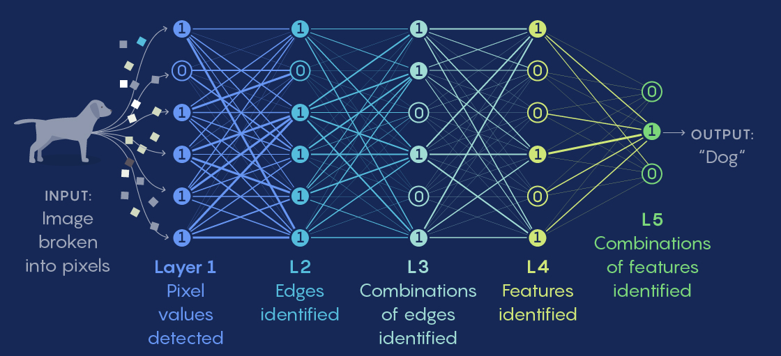
Rosenblatt creates elementary mathematical functions that he calls neurons: these neurons take in several signals, combine and transform them to produce a single output channel. If the sum of all these signals exceeds a certain threshold, the neuron activates and outputs the sum; otherwise, it outputs 02. A connection can be formed from the output of one neuron to the input of another, thus forming successive layers, with a particular weight assigned to each connection. For example, let’s build a neural network to detect which animal is present in an image. Neuron a on layer 1 detects proposition A, for example “orange color”, and neuron b on layer 2 detects proposition B, “the image shows a fox”. In this case, we want the connection from neuron a to neuron b to be positive: if we detect an orange color, as it is likely that an orange animal is a fox, there will be a positive signal to help B activate as well. Conversely, if neuron c on layer 2 detects condition C, “the image shows an elephant”, we prefer the connection from a to c to be negative: if the image is orange, it is probably not an elephant. Each successive layer can thus rely on the previous ones to move up a level of abstraction: if layer 0 is the direct signal from the pixels, layer 1 represents elementary colors and shapes, layer 2 can already represent more advanced patterns and shapes, layer 3 can represent concepts like “claw” or “ear”, and layer 4 can determine which animal it is. This approach is the first draft of today’s large models.
Universal Approximators
If we only connected neurons that sum signals with certain coefficients, we would obtain a linear system: that is, by multiplying all input signals (e.g., pixel values) by the same coefficient, the output would also be multiplied by that coefficient. Such a network would not be very useful: in our image classification example, if we halve the brightness of the image, thus the value of each pixel, the value of the output neuron would also be halved, so the classification “this is a cat” would become half as certain, which would be absurd: at night, cats might be gray, but they remain cats. The key to the effectiveness of neural networks lies in the nonlinear function applied to the sum at the neuron output: this is what gives the neural network its non-linear character. In fact, a neural network is a universal approximator: it can reproduce any function of its inputs as finely as desired, provided it has enough intermediate layers and that its weights are correctly adjusted.
The AI Winter
Rosenblatt’s approach, called “connectionist” because it relies on the connection of many simple elements, enjoys initial success and flashy publicity3, but quickly faces criticism.
Indeed, this network model can work, but how to determine the connection weights? If we have to manually adjust each connection weight to get a good result on our problem, it will be extremely costly to adapt the network to each new problem or data point. This is a crucial problem: learning.
It is this limitation that leads to the downfall of the connectionist approach.
For years, another approach takes over: the symbolic approach. The symbolic approach seeks to create reasoning from the other side: starting from a high level of abstraction. This school aims to represent all possible reasoning in a symbolic language. Once the situation is expressed as a sentence in this symbolic language, it would become simple, using predetermined calculation rules, to transform the sentence into a logical conclusion. This approach is theoretically appealing because it is more explainable. But it is extremely ambitious: is it possible to express all the decisions we make, even those made mechanically4, in a theoretical language? Because this language would have to be able to accurately express all the concepts of the world, and even the imaginary ones. Moreover, such an AI would have discrete reasoning processes: the inputs could only be symbols present or not, hence 0s or 1s. But aren’t many of our reasonings a fuzzy sum of continuous parameters? For example, when I decide whether to go out or not, I consider the weather: but the color of the sky varies continuously across all shades of gray to blue, and removing this nuance would certainly reduce the quality of reasoning.
To mitigate the difficulty induced by this complexity, the symbolist community starts by developing expert systems restricted to a specific domain. But they are very costly to design for poor performance: this approach yields little fruit. And so begins what has been called the “AI Winter,” a long period of stagnation and doubt.
Yann LeCun, Geoffrey Hinton and Backpropagation
In science, revolutions often begin at the margins. In the 1990s, the young Yann LeCun starts to take an interest in Artificial Intelligence. He reads the account of a debate where the linguist Noam Chomsky asserted that the brain had pre-established structures for learning to speak. Opposite him, the developmental psychologist Jean Piaget argued that everything is learned, even some of the language structures, and that language construction occurs gradually throughout the development of intelligence5. Who is right: does reasoning occur from pre-constructed structures, or can it emerge from simple mechanisms? This question will be formative in the development of Artificial Intelligence. Yann LeCun henceforth makes learning his guiding principle.
He revisits Rosenblatt’s neural networks and revives a gradient backpropagation technique that had existed since the 1960s in control theory6 but was seemingly ignored by Rosenblatt, recently re-theorized by Rumelhart and Canadian Hinton, which theoretically allows training a multi-layer neural network, i.e., adapting it to a dataset. LeCun consolidates the theory7 and achieves for the first time a model capable of learning from a dataset. He applies it to recognizing digits in photos of handwritten digits, compressed to 28x28 pixels8. The demonstration is impressive, much better than all existing systems at the time. By the late 1990s, his system processes 10 to 20% of all checks in the United States.
Prediction Problems: Classification and Regression
There are several formulations of problems one might want to solve with Artificial Intelligence. We always want to predict an output based on an input – each of the latter may have one or more elements. If the output is discrete, meaning it must belong to a finite number of categories, it is called a classification problem. For example, if we ask, “What type of animal is that?” by inputting a photo of an animal (which is a set of unique pixels), it is a classification problem. Regression is the configuration where the output can take continuous values along an axis: for example, “all values between 0 and 1.” The question “How much is the NVIDIA stock worth at time t?” is a regression question. In the example of Yann LeCun’s tool mentioned above, the goal is to predict a digit between 0 and 9: it is therefore a classification problem.
Learning, Then Inference
Yann LeCun was among the pioneers of AI learning. Today, the two fundamental steps of Artificial Intelligence are: learning and inference. It is important to always keep this distinction in mind. Learning is the stage where we adjust the model’s weights to give it reasoning ability, while inference is where the model predicts an outcome based on its inputs.
When we talk about training or optimization, it is the learning stage. When we talk about prediction or generation, it’s inference.
Take the example of ChatGPT. It is a product (a chatbot) offered by OpenAI, powered by one of their models, for example, GPT-4. Training is prodigiously expensive – millions of euros – and lasts months. This is why the model’s “knowledge” (we will see later that this knowledge is extremely fuzzy) stops at a certain date: yesterday’s information cannot yet be integrated; it would take at least a few weeks to retrain the model with this information.
On the contrary, when a user chats with the chatbot, it’s only inference, much faster (a few milliseconds) and less expensive (a few thousandths of a cent). The model does not learn from what we tell it – it may seem to remember because it generates its text from the entire conversation from the beginning, but as soon as the conversation changes, it starts over. However, the conversation could very well be saved as material for the training datasets of OpenAI’s future models.
⚙️ Technical Building Block: Training by Backpropagation
How to change the connection weights of a neural network to make it perform well on a problem? For example, starting from a network with weights initialized randomly, how to train it to recognize the animal in a photo? We start by adding a final layer of neurons to the network, with as many neurons as possible prediction classes. For example, we can train the network to recognize only 1. A cat, 2. A dog. We, therefore, add a final layer of 2 neurons: if neuron No.1 activates with a higher value, the prediction is “a cat”; if it’s No.2, it’s a dog. Of course, at this stage, since the weights are created randomly, the predictions will be random. We then want to train the network, i.e., adjust its weights to get correct predictions.
For this, we need a dataset containing animal photos annotated with the name of each animal. For example: (photo_1193.jpg, “a cat”). Then (photo_2194.jpg, “a dog”), etc.
We must therefore find the parameters (here the connection weights) that minimize the error (the number of wrong predictions). For this, we will modify all our parameters in small steps. At each step, we will:
- Take a new example from our dataset, which is a photo - animal name pair.
- Calculate the prediction for the given image. Then, compare it to the real animal name: is the prediction wrong or correct?
- If it is correct, we reward the weights that helped predict it by reinforcing them; if it is wrong, we must penalize the weights responsible by diminishing them. To execute this adjustment and distribute the responsibility of an error or success among all weights, we backtrack from the end of the network: this is the backpropagation operation.
This operation is repeated hundreds of thousands of times: this is the optimization process, which will gradually converge to a better weight configuration giving good predictive performance to the model.
This algorithm has undergone some tweaks since then, but it is still the same one that underpins all of Artificial Intelligence today.
⚙️ Technical Building Block: Optimization - Finding the Lowest Valley
A bit too many barbarisms here, isn’t it? Don’t worry, after this technical point, I’ll leave you in peace for a few pages! And we’ll explain below why deep neural networks are harder to train than other AI algorithms.
To do our optimization, you saw just above that we took a small step via backpropagation. But let’s try to better understand what’s happening.
Let’s revisit the problem of training a neural network.
What do we want to achieve in the end? We want to obtain the best set of parameters in the network, the one that gives us the smallest average error on our training dataset.
We call this average error the “cost function”9: “cost” because the error is a cost we want to minimize, and “function” because this average error varies depending on the parameters: when we vary each parameter, the average error varies accordingly.
Now, how to find the best set of parameters to minimize this cost function? To simplify the problem’s representation, let’s take a network with two parameters, a and b. Of course, this is a drastic simplification of reality where models have billions of parameters. But it is practical because we can represent the cost function on a 3D graph: we note parameter A along the X-axis, parameter B along the Y-axis, and the network’s cost function (which thus depends on parameters A and B) along the Z-axis.
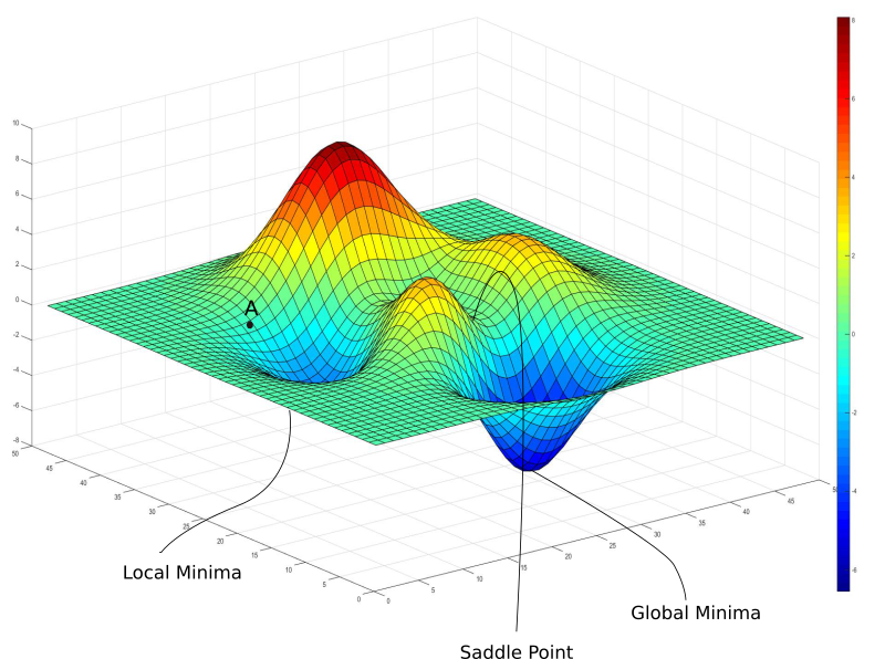
The cost function varies depending on its two parameters: we get a nice landscape.
Note, this graph has nothing to do with the previous one: here, the X and Y axes represent parameters, while in the previous one, X and Y were system inputs. The only commonality between these two graphs is being in 3D.
What do the mountains and valleys of this landscape signify, and what place do we want to find?
The mountains correspond to sets of parameters for which the network is poor since its average error is high. Conversely, the valleys are local minima, corresponding to good sets of parameters that minimize the error. Our goal is therefore to find the deepest of all valleys, the global minimum.
Since our parameters A and B were initialized randomly, the initial placement in the landscape is random. The whole point of optimization is to find the deepest valley starting from this point.
Why not directly calculate the global minimum? Well, with pleasure, but how? The landscape we have drawn here is simple; we could grid it into a grid of 20 values on each axis, we would have 400 combinations to test, and it would be done. Yes, but remember that we have greatly simplified the problem: in reality, networks often have millions of parameters. For a million parameters, with 20 values on each axis, there would be 20*1,000,000 parameter sets to test; we would still be there for centuries.
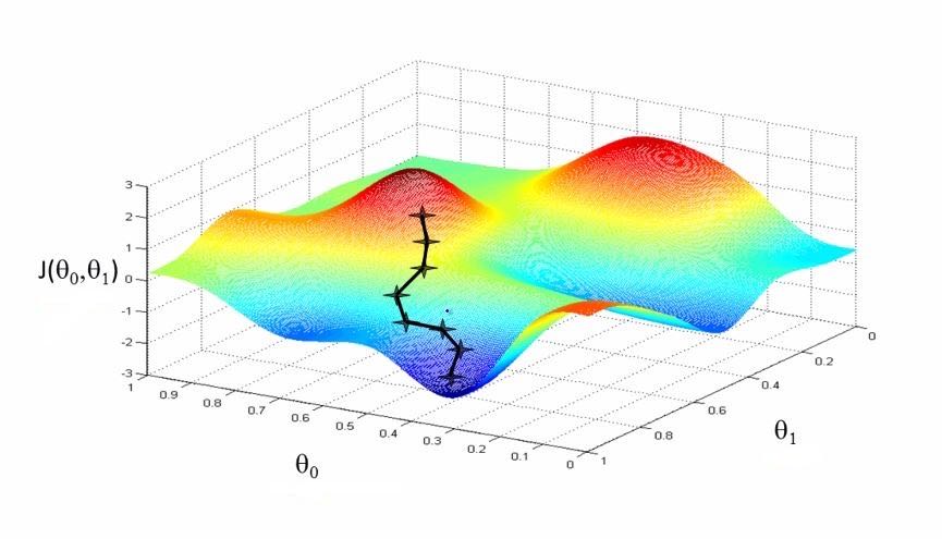
We are therefore in the situation of a mountaineer lost in a snowstorm, seeking to reach the valley bottom but unable to see a meter ahead.
Hence the backpropagation technique. We take examples one by one: for each example, we take the direction given by gradient backpropagation and take a small step in that direction: this corresponds for the mountaineer to taking a small step downhill. And little by little, gradually descending the slope like a ball rolling driven by gravity, we hope to find the bottom of the deepest valley.
Could we not get stuck in a basin (a local minimum) or stopped in balance on a ridge? Surprisingly, it works: most of the time, this method allows for a long descent and finding a very good minimum.
This algorithm has been improved since then – for example, we add inertia to the ball to prevent it from stopping at the first basin – but it remains very similar.
However, for LeCun and Hinton, who had begun a collaboration, winter was still not over. A new algorithm, the SVM, similar to a single-layer network, works very well on small datasets and does not require a complex training procedure. The training procedure for their “deep” neural networks is more complex and lacks a theoretical guarantee of success10, so it is judged less elegant. As a result, deep neural networks are once again sidelined by the AI community.
Deep Learning Makes a Name for Itself
What will really change the game is the arrival of massive datasets and the development of GPUs, processors specialized in matrix multiplication that allow neural networks to train on enough data to reveal their power. Yann Lecun now works with Geoff Hinton and Yoshua Bengio at the Canadian Institute for Advanced Research (CIFAR): this trio of the “neuron conspiracy” does not give up and convinces a growing fringe of researchers. Every year, major machine learning conferences bring together researchers from around the world: this is a valuable opportunity to showcase their ideas and results. In 2007, the NeurIPS conference rejected the workshop proposed by the trio without explanation. No problem: they organize a pirate workshop funded by CIFAR, chartering their own bus to bring participants. And it’s a success: their workshop attracts 300 researchers, making it the most attended at the conference! This event marks the adoption of the term “deep learning,” coined a year earlier by Hinton, in the specialized press11.
Deep learning gradually establishes itself, particularly in image processing. Starting in 2009, the vision research community tries to reduce its errors on a huge test bench called ImageNet: 12M images to classify into 22k categories, created by Fei-Fei Li, director of the SAIL lab at Stanford.
In 2012, at the ECCV conference, Alex Krizhevsky, Hinton’s student, unveils his network called AlexNet. In front of a packed room, he announces that he has beaten the world’s best model, with half the errors! Gradually, neural networks take the top spots on all benchmarks. Richard Sutton described this as a “bitter lesson”: all the most sophisticated approaches to trying to reproduce how we think are far outdone by simple stacks of neurons, provided they are trained with enough data and computing power. But let’s continue following Yann LeCun: carried by the success of deep learning, he is hired by Mark Zuckerberg to launch AI research at Meta (then Facebook). He is the one who has pushed Meta’s major effort to offer open-weight models, meaning models with publicly available weights and architectures.
Generalization and Ockham’s Razor
But let’s take a step back. We have seen above how two essential characteristics of neural networks were constructed: neural networks are universal approximators, meaning systems that can reconstruct any function from their inputs, and they can learn through LeCun and Hinton’s backpropagation. But such a system will not necessarily be useful. For example, a dictionary has inputs – the defined terms – and outputs – the definitions. We can associate any definitions we want with the dictionary’s terms: it is, therefore, a universal approximator.
It also allows for learning: we can edit the definitions, as Larousse and Petit Robert do every year.
But yet, as soon as we want to look up the definition of a term that is not there, the dictionary is of no use. However, for real problems, we want to give the model an input it has never seen in training and still get a correct prediction. For example, in our classifier that determines the animal in a photo, we want a dog photo always to yield the prediction “dog,” even if the dog in question belongs to a breed the classifier has never seen during its training.
In other words, we want our model to generalize the information from its training data through proto-reasoning like “if there is a triangular snout rather than a trunk, it is probably a dog.”
A risk of a naive universal approximator is to adapt to the data without really generalizing. This is called “overfitting.” See the figure below for an illustration of this phenomenon: the model learns a boundary that is far too complex between its classes and, as a result, proves useless as soon as we move away from the examples in its training.
![Several models try to predict based on coordinates [Latitude, Longitude] the output 'Is located in France'. They predict 1 for 'Yes', 0 for 'No'.](/assets/images/2024-08-15-brief-history-of-ai/france_graph_en.png)
We want to learn the right way, by generalizing.
This is a difficult problem. The best way we’ve found is to seek simplicity, thus following Ockham’s Razor. This methodological principle was formulated by the English Franciscan monk William of Ockham: “Plurality must not be posited without necessity”12. To explain a phenomenon, it is better to simplify things by first considering the explanation that involves the fewest factors, as it is the one with the least strong hypothesis. We often unconsciously use this principle: for example, even if a student arriving late to an 8:30 am math class can explain their tardiness by a complex set of circumstances, the teacher might think that the student simply overslept.
It is this search for simplicity that automatically invalidates most conspiracy theories: if global warming were a conspiracy, it would require incredible coordination between thousands of actors across the planet: meteorologists, farmers, biologists… It is much simpler to consider that the climate is actually warming, even if admitting this thesis implies unpleasant consequences. This principle is so powerful that it was described by the philosopher Bertrand Russell as “the supreme methodological maxim when philosophizing”13.
Several principles of deep learning can be directly justified by Ockham’s Razor: among others, regularization. This involves adding a tendency during model training for all weights to approach 0. Thus, a weight not prompted by backpropagation to grow to favor a certain output over another – and if it is not affected by backpropagation, it is useless – will naturally tend towards 0. This simplifies the model’s decision boundaries and empirically helps generalization a lot.
To recap: we want our model to be able to finely approximate the training data while keeping decision boundaries simple enough to generalize. This is a delicate balance to find and a significant part of the art of machine learning.
Meta-Intelligence: Designing Structures That Learn
Remember Richard Sutton’s “bitter lesson,” which said that the effort we put into building sophisticated reasoning structures was of little use compared to the brute computing power launched on millions of examples: now reread the paragraph above on regularization, which shows that giving the machine the right mechanisms can help its learning. Isn’t this a contradiction?
In fact, these two extracts do not contradict each other because they pertain to different levels of learning. Sutton’s statement applies to the basic level, that of reasoning: dictating reasoning to the machine is inefficient. But if we rise a level conceptually, we can give the model the right structures to learn effectively on its own during training. In other words, we don’t explain in detail the method to solve each problem but provide the machine with the necessary conditions to find this method during its learning. This is the essence of today’s Artificial Intelligence, and it is what I find immensely enjoyable about this work: there is a demiurgic aspect to preparing all the necessary learning conditions, then launching this learning and watching the optimization happen.
Attention
Image classification gradually becomes a solved problem: convolutional neural networks overcome the most challenging benchmarks, and they can already assist radiologists in detecting cancerous tumors.
But text processing remains out of reach.
In 2013, the Word2vec algorithm allows for creating word representations as vectors, and with word representation as vectors, we can begin to translate texts14.
⚙️ Technical Building Block: Representing Words as Vectors
First, what is a vector? It’s simply a list of numbers in a precise order. For example, coordinates in space in X, Y, Z form a vector in three dimensions that can be noted [X, Y, Z]. Conversely, any vector can be seen as the coordinates of a point in space. In one, two, or three dimensions, we can visualize them: but vectors have no size limit; they can be a thousand dimensions.
We can perform operations on vectors: for example, for two vectors of equal size, we can multiply each number in one by the number in the other at the same position (for the same dimension), then sum all the products to get a single number. This operation is called the dot product. We can also, of course, add or subtract them by performing the addition or subtraction on each dimension one by one.
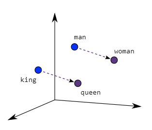
An idea that emerged early on was to represent words as vectors: the dimensions could represent concepts, for example, the feminine-masculine axis, big-small, rainy-sunny, strong-weak…
This approach was implemented by the Word2vec algorithm in 201315, which creates a vector representation for over a billion English words. This representation is fascinating: the obtained vectors have mathematical relationships that reproduce conceptual links between the words they represent. For example, if we take the vector representing the word “queen,” subtract the vector of “woman,” and add “man,” we get the vector for “king”! Thus, we realize that word vectors represent concepts like royalty or femininity.
To do this, we can place the different vectors representing the words of a sentence side by side and input the whole thing into a large neural network to ask it to predict the word to complete.
However, until 2017, deep neural networks were not really capable of considering dynamic interactions between their different inputs.
To illustrate this difficulty, let’s take the example of German => English translation.
In German, the verb is pushed to the end of relative clauses, even if the subject remains at the beginning16.
“Ich frohe mich, dass er am Donnerstag Abend zum Essen kommt.”
“I glad myself, that he on Thursday evening to dinner comes.”
But this is not the case for a non-relative clause:
“Er kommt am Donnerstag Abend zum Essen, ich frohe mich”
“He comes on Thursday evening to dinner, I glad myself.”
So depending on the content of the sentence, whether or not the sentence is formulated as a relative clause, the position of the inputs is completely altered. We would therefore need to model dynamic interactions according to the inputs, such as “if we are in a relative clause, the subject of the clause must interact strongly with the very last word (the verb).”
But our neural network is not capable of this because it processes its inputs only according to their position: whatever the input sentence, the first word will always be taken into account in the same way in the network: by arriving in neuron No.1 of the first layer, it will then be sent to all the neurons of layer 2 according to the network’s pre-established weights, and so on for all the layers.
The key to this problem was found in 2017 with a new component: self-attention: the article Attention is All You Need, which has since been cited in over a hundred thousand other articles, proposed a new model architecture named Transformers, which beat the best models of its time while being 100 times less costly to train. The main innovation was the adoption of an existing component, attention, applied in a clever way: self-attention of the input sentence was calculated towards itself: this allowed transforming the representation of each word to incorporate a bit of the representation of the words linked to it. In our German sentence above, “dass” (that) would take a bit of the representation of “er” (he) and a bit of “kommt” (comes), even if these words are at opposite ends of the sentence. Self-attention layers are inserted into the network at regular intervals.
Remember that going up in the network layers creates increasingly abstract concepts: adding self-attention layers to high areas means that in addition to allowing distant words to interact in the lower layers (“the verb must agree with its subject”), attention allows distant concepts to interact in the higher layers (“the second idea of this sentence is related to the paragraph title”). Thus, the model is enriched with additional interactions at all levels of abstraction.
A Transformer-Based Decoder
Let’s see how a Transformer architecture is used to generate text. We start from an initial sentence, usually the user-provided prompt.
The words of the sentence are transformed into vectors. Well, not exactly the words. It’s better to split the sentence into “tokens”17, which are a subdivision of words into smaller units.
Splitting into tokens reduces the necessary vocabulary (since they are short, the set of tokens is smaller than that of all words) and also allows for similarities between words. For example, the suffix “tion” indicates an action or the result of this action in French: considering “tion” as its own unit will allow the LLM to recognize the associated concept, whatever the word with “tion” present, even if it is a neologism unknown to the model such as “tokenization.”
Each token is thus transformed into a vector. Then these vectors pass through the Transformer architecture, which is a stack of Transformer blocks, each composed of a self-attention layer, then a classic layer called “Feed-forward.” The last layer of the network contains N neurons, with N being the vocabulary size (these are subword tokens, not complete words). We note i as the number of the neuron with the highest output value: it is thus the i-th token of the vocabulary that is chosen.
This token is then added to the other tokens. And thus, we obtain a new sentence, which corresponds to the initial sentence, augmented by a new token. The whole process is then rerun using this augmented sentence as input to add yet another new token. And so, step by step, we extend the sentence until the generated token is a specific token,
Learning Methods
We classify several learning methods based on the data used.
Supervised learning: this is the one used in our image classifier example. It means that we have created a dataset where each example has been annotated. For example, “image 1 is a dog,” “image 2 is a cat.” These are often datasets rich in information for the model but very costly to produce when millions of examples are needed!
Unsupervised learning: a more economical solution is to train the model on unannotated data. But most models cannot be trained this way: how to find out if the prediction is correct or not when there is no reference? If models can be trained using this method, it’s a chance. “Clustering” methods, which take a set of vectors and group them into “clusters,” can work unsupervised. And luckily, decoder architectures can too! See the example given above.
Reinforcement learning: when we don’t even have a dataset, we can use reinforcement learning. This method is widely used in robotics, where the dimension of possible outputs is immense: unlike the image classification example where the prediction is chosen from among a dozen classes, for a robotic arm with five degrees of freedom performing a movement for ten seconds, the field of possible trajectories is immense, making a pre-built dataset much less useful. It’s an entirely separate field that involves complex optimizations.
So for now, we have kept the Decoder, which generates its response token by token, even if it invents fanciful answers when it has nothing coherent to complete. This last case is called hallucinations: the model gives a probable but completely invented answer.
For example, to the question “How much does a cow egg weigh?”, some models will immediately complete something like: “How much does a cow egg weigh? A cow egg weighs between 2 and 5 kilograms, depending on the breed of the cow.
Scaling Up: Large Language Models
In October 201818, a new thunderclap in the research world: Google researchers (again) publish BERT, a Transformer-based architecture that beats the best models on 11 different tasks. Usually, beating a benchmark is already worthy of publication: beating 11 is a resounding achievement! How did they do it? They used the Transformer architecture with very few modifications, only with well-done training, and up to 24 layers stacked instead of 6, bringing the model to 340 million parameters – huge for the time.
This is the start of a gold rush: everyone wants to use BERT’s architecture. Facebook publishes a few months later RoBERTa, where they mock Google researchers by taking their model with a strictly identical architecture but training it better to achieve superior performance. Microsoft will publish its version, DeBERTa, a year later with a modified architecture. Then, as the results obtained by the models continued to improve as their number of parameters increased, models were trained on an increasingly larger scale. Thus, we talk about Large Language Models (LLMs).
In fact, what stunned researchers at that time was a principle already mentioned by OpenAI researchers in 201719, a year before they published their first GPT (for “Generative Pre-trained Transformer”). The project involved performing “sentiment analysis,” i.e., interpreting whether the general opinion expressed by a short text is positive or negative. This is a task on which researchers have spent decades creating large datasets, manually annotating thousands of user reviews collected from commercial sites. In contrast, OpenAI’s 2017 project aimed to train a model simply to predict the text of a user review, letter by letter (we were not even at the token level yet). Once this model was trained to predict the text, the researchers realized it was excellent at sentiment analysis, despite never being trained for this specific task. This is an example of the “transfer learning” phenomenon: a model’s learning on a specific task also improves its performance on another task.
The most commonly given explanation for this transfer learning phenomenon is that training to model text gives the model a powerful statistical representation of language, making it more effective in other tasks. There is still a very lively debate about whether these models truly understand language, as well as the social and physical phenomena it represents20: some argue that during their learning, models develop a real internal model of the world. Probably not a model close to what we would envision – if we have a common one at all – but a useful model nonetheless.
Thus, many so-called “emergent” properties have been discovered as larger and larger models were trained, unpredictably. For example, by pre-training a model increasingly large on the same text corpus, it was found that beyond a certain size, it gradually goes from ~0 to ~100% performance on a completely ancillary task.
A striking example is GPT-4’s technical report21, which shows dozens of exams where the model has become much better without being trained on these exams22.
It has been shown that this sudden unlocking of new abilities is the natural result of an incremental increase in LLM performance23. To draw an analogy in the real world: if I run the marathon in 10 hours, I won’t win any championships. And gradually reducing my time, 10 minutes by 10 minutes, still won’t affect my medal count… Until the three stages between 2h30 and 2h, where I will suddenly go from a departmental performance to that of a world champion. Of course, for us humans, these last ten-minute slices are the hardest to achieve – because we all start with the same equipment (our body), and the effort to change it is immense. But for a machine whose architecture can be modified at will, the 2h threshold is no harder to pass than the previous ones. A notable result: the emergence of each of these abilities from a certain model size is unpredictable.
Since 2017, a few significant innovations have further improved Large Language Models: massive and higher-quality training data, grouped-query attention24, position encoded by rotation matrices25, SwiGLU activation26… But the foundation remains the same: a Transformer architecture. Only, more and more neuron layers, neurons per layer, and attention heads are added to the networks. Pre-trained LLMs on increasingly vast text corpora have gradually taken the top spots on all possible tests, in all tasks and all modalities. It seems we may have found a universal recipe for intelligence.
-
Permitted by the architecture conceived by von Neumann in 1945 and implemented for the EDVAC in 1952, which separated for the first time the software from its mechanical support (hardware), allowing coding without concern for mechanics. ↩
-
The mechanism described here is that of the ReLU function, but many others have been constructed. Today, SwiGLU is used in Meta’s Llama-3 models. But this will probably change someday! ↩
-
The New York Times wrote in 1958 that it was the “embryo of an electronic computer that the Navy hopes will walk, talk, see, write, reproduce itself, and be aware of its existence.” ↩
-
On this topic, see Hubert Dreyfus’ critique, based on Heidegger’s Ready-to-hand and present-to-hand. ↩
-
Y. LeCun, Quand la Machine apprend. ↩
-
H. J. Kelley, “Gradient Theory of Optimal Flight Paths”, ARS Journal, vol. 30, nᵒ 10, p. 947‑954, Oct. 1960, doi: 10.2514/8.5282. ↩
-
For those who want to train technically, I recommend reading the paper written by LeCun on the subject, https://yann.lecun.com/exdb/publis/pdf/lecun-88.pdf. He lucidly re-demonstrates all the equations leading to backpropagation. ↩
-
This is the MNIST dataset:
“MNIST handwritten digit database, Yann LeCun, Corinna Cortes and Chris Burges” [Online]. Available at: https://yann.lecun.com/exdb/mnist/ ↩ -
In English, “loss function,” often abbreviated as “loss.” ↩
-
If the average error made by the network is plotted against its parameters, a non-convex function is obtained. Training involves finding the global minimum of this function, but due to this non-convexity, it is not guaranteed that backpropagation will find it. ↩
-
Y. LeCun, Quand La Machine apprend. ↩
-
In Latin: Pluralitas non est ponenda sine necessitate ↩
-
B. Russell, On the Nature of Acquaintance, p. 1456 ↩
-
The first effective networks for text translation were the Recurrent Neural Networks (RNN) ↩
-
T. Mikolov, K. Chen, G. Corrado, and J. Dean, “Efficient Estimation of Word Representations in Vector Space”, Sept. 6, 2013, arXiv: arXiv:1301.3781. doi: 10.48550/arXiv.1301.3781. ↩
-
This may be why German political debates are less interrupted and seem more respectful: because it’s hard to know what your opponent is saying until they finish their sentence! ↩
-
This process bears the sweet name of “subword tokenization.” ↩
-
Date of publication on the Arxiv website, where papers can be published very quickly without going through the long validation processes of journals or conferences. By the time it was published at the ICLR conference in May 2019, their paper already had 600 citations! ↩
-
A. Radford, R. Jozefowicz, and I. Sutskever, “Learning to Generate Reviews and Discovering Sentiment”, April 6, 2017, arXiv: arXiv:1704.01444. doi: 10.48550/arXiv.1704.01444. ↩
-
M. Mitchell and D. C. Krakauer, “The Debate Over Understanding in AI’s Large Language Models”, Feb. 10, 2023. doi: 10.1073/pnas.2215907120. ↩
-
OpenAI et al., “GPT-4 Technical Report”, March 4, 2024, arXiv: arXiv:2303.08774. doi: 10.48550/arXiv.2303.08774. ↩
-
Be careful though: at these scales, it is necessary to train the models with massive training data, collected without too much discrimination across the entire Internet. It often happens that the answers to certain tests have already been seen by the models during their training and memorized, which distorts the test. This is referred to as “contamination” of the test dataset. ↩
-
R. Schaeffer, B. Miranda, and S. Koyejo, “Are Emergent Abilities of Large Language Models a Mirage?”, May 22, 2023, arXiv: arXiv:2304.15004. doi: 10.48550/arXiv.2304.15004. ↩
-
J. Ainslie, J. Lee-Thorp, M. de Jong, Y. Zemlyanskiy, F. Lebrón, and S. Sanghai, “GQA: Training Generalized Multi-Query Transformer Models from Multi-Head Checkpoints”, Dec. 23, 2023, arXiv: arXiv:2305.13245. doi: 10.48550/arXiv.2305.13245. ↩
-
J. Su, Y. Lu, S. Pan, A. Murtadha, B. Wen, and Y. Liu, “RoFormer: Enhanced Transformer with Rotary Position Embedding”, Nov. 8, 2023, arXiv: arXiv:2104.09864. doi: 10.48550/arXiv.2104.09864. ↩
-
N. Shazeer, “GLU Variants Improve Transformer”, Feb. 12, 2020, arXiv: arXiv:2002.05202. doi: 10.48550/arXiv.2002.05202. ↩